Lab 9: Object Based Classification

Goals and Background

The main purpose of this lab is to gain knowledge in performing object-based classification within eCognition.  eCogniton is a computer program which only performs object-based classification of satellite images. Object-based classification is a somewhat new form of classification in the world of remote sensing.   In this lab I will learn the step required to perform object-based classification.  I will be using two different classification methods which include, random forest classifier and support vector machine classifier.

Methods

I performed both forms of classification on the same image of the Chippewa and Eau Claire County in Wisconsin from previous classification labs.  The classification process was performed in eCognition as stated above.  Additional programs will be noted for there uses.

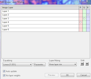
I imported the image provided to me utilizing Import Image Layer after creating a New Project. The resolution was set to 30 /pxl and the Use geocoding box was selected. The image was displayed in an unfamiliar color scheme.  I utilized Edit Image Layer Mixing to change the color display to a familiar 4,3,2 band combination (Fig. 1).

(Fig. 1) Edit Image Layer Mixing window set to display a 4,3,2 band combination image.

Segmentation and Sample Collection

I created a new process in the Process Tree after opening from the Process menu.  The first “process” acts like a label/heading to build the “tree” from. From the first process I created a New Child which I labeled Generate objects.  The step will be creating segmentation with in the image.  Segmentation groups like features based on pixel value, texture, and compactness. In the edit window I set the Algorithm to multiresolution segmentation along with setting Shape to .3 and Compactness to .5. per the instruction of my professor.  The setting for shape and compactness were derived from trial and error from previous work my professor has done. I selected Execute after assuring all of my parameters were set correctly. The image was now displayed with the created segmented areas (Fig. 2).

(Fig. 2) Zoomed in image with the segmentation layer over top of the satellite image.

Creating training samples is the next step of the classification process. For this lab I will be creating classification for the following classes:

• ·         Forest
• ·         Agriculture
• ·         Urban/Built-up
• ·         Water
• ·         Green vegetation/shrub
• ·         Bare soil

Using Class Hierarchy and Insert Class I was able to create classes and label them with a corresponding color (Fig. 3). Take from Lab instructions if needed). With the classes created I was able to start collecting samples using Select Samples from the Classification menu and Samples sub-menu. I zoomed and panned around the image selecting areas which were homogeneous with forest areas after selecting Forest from the classes list. After selecting an area the segmented area would change to the color corresponding to the class (Fig.4*****************).  After collecting the required number of samples (specified by my professor) for the forest areas I utilized the same process for all the remaining classes.

(Fig. 3) Class list created for classification.

(Fig. 4) Image of sample areas selected with appropriate color displayed.

Implement object classification

I created a Scene Variable from the Manage Variable window found under the Process menu. The scene variable is like setting environments in ArcMap as it gives a location for the processing to store information.

I Appended New process labeled RF Classification below the segmentation “Level 1” step. I then inserted a New Child to the new process. The new child process was labeled Train RF Classifier.  Within the Edit Process window I set a number of parameters to properly execute the training classification (Fig. 5).  The parameters again were given to me from my instructor based on his experience with the RF Classification. The training samples were brought in to the classifier window through the Feature drop down in the Edit Process window. The Select Features window opens after selecting <select features…> from the drop down menu. I added selected parameters from my trainings samples within the window per the advice of my professor (Fig. 6*************). The final step is to implement/perform the classification. I inserted a child to RF Classification labeled Apply RF Classifier. The parameters were set in the window to properly apply the previous steps to the image (Fig. 7*****).  Select the View Classification icon after Executing the apply step of the process.

(Fig. 5) Edit Process window with parameters set to train the RF classifier.

(Fig 6) Select Features menu with training data selected.

(Fig. 7) Edit Process window applying the RF classification.

(Fig. 8) Process Tree after imputing all of the processes to perform RF Classification.

Export to Erdas

Utilizing Export Results from the Export tab I created an Erdas Imagine Image.  I opened the image in Erdas Imagine to alter the color scheme of the classification to match previously completed classifications. 

Support Vector Machines

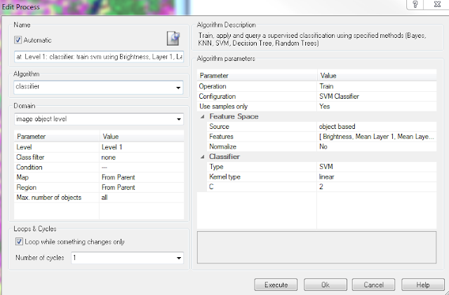
Support Vector Machines (SVM) is another learning algorithm which utilizes a hyperplane to perform classification of segmented areas.

I utilized the same steps above to perform the SVM classification on the same segmented image. The only difference is the parameter settings when training the classifier (Fig. 9). The parameter setting were again provided to me by my professor in the lab instructions.

(Fig. 9) SVM classification parameters set in the Edit Process window.

Results

Both classification results had some error when comparing the produces map with Google Earth. The areas with errors could have been corrected using Manual Editing in eCognition.  The likely reason for the error is from incorrectly selected training samples. The SVM classification produced more accurate results compared to the RF classification from my observations.

Sources

Lta.cr.usgs.gov,. (2016). Landsat Thematic Mapper (TM) | The Long Term Archive.