Thursday, May 5, 2016

Lab 12: Radar Remote Sensing

Goals and Background

The purpose of the lab is to provide me with the basic knowledge of performing preprocessing and processing operations of remotely sensed radar imagery. Radar interpretation is considerably different than conventional remote sensing. Radar is more closely related to Lidar due to the active sensor which emits a beam and receives a return signal. All radar imagery is collected off nadir so image correction is a must. The topics covered in the lab include:

  • noise reduction through speckle filtering
  • spectral and spatial enhancement
  • multi-sensor fusion
  • texture analysis
  • polarimetric processing
  • slant-range to ground-range conversion
Methods

The first half of the methods was performed in Erdas Imagine.  The second half was performed in ENVI software (I will note when the switch was made).

Speckle filtering

Speckle filtering reduce the salt and pepper noise on a raw radar image. I was provided an image by my professor for the following steps (Fig. 1).

(Fig. 1) Original radar image provided for the lab.


I selected the Radar Speckle Suppression from the Utilities sub-tab from the Raster tab. I set the parameters in the Radar Speckle Suppression window to the following:
  • Coef. of Var. Multiplier = .5
  • Output Options = Lee-Sigma
  • Coef. of Variation = .275 (This value was calculated by selecting Calculate Coefficient of Variation in the Radar Suppresion dialog box and viewing the results in View Session Log found in the Session sub-tab of the File menu.
  • Window Size = 3x3
  • The remaining parameter were left as the defaults
I then selected ok to run the speckle suppression. After the first speckle suppression I ran another speckle suppression on the resulting image and then again on the second result.  The parameters for each suppression was set to the following:

   Speckle Suppression of 1st result
  • Coef. of Var. Multiplier = 1.0
  • Output Options = Lee-Sigma
  • Coef. of Variation = .195
  • Window Size = 5x5
  • The remaining parameter were left as the defaults
   Speckle Suppression of the 2nd result
  • Coef. of Var. Multiplier = 2.0
  • Output Options = Lee-Sigma
  • Coef. of Variation = .103
  • Window Size = 7x7
  • The remaining parameter were left as the defaults
One way to evaluate the effectiveness of the speckle suppression is to analyze the histograms of the images.  The histograms should become less jagged after each successful suppression pass (Fig. 2).

(Fig. 3) Display of the histograms as the become less jagged through speckle suppression.


Edge enhancement

I performed edge enhancement on the original image and the result of the 3rd speckle suppression.

The edge enhancement is performed by selecting Non-directional Edge from the Spatial sub-tab of the Raster tab. The only parameter I set was the Output Option was set to Prewitt. The remaining perimeters were left alone.

Image enhancement

There are numerous image enhancement functions provided in Erdas Imagine. I will be utilizing the Wallis Adaptive Filter for this portion of the lab.  I will be utilizing an image provided to me by my professor (Fig. 3).

(Fig. 3) Original radar image I utilized to apply the Wallis Adaptive Filter.

Opening the Radar Speckle Suppression as I did in previous steps I changed the Filter to Gamma-MAP. I then opened Adaptive Filter from the Spatial sub-tab from the Raster menu. Using the result from the Gamma-MAP suppression as the input file, I checked the Stretch to Unsigned 8 Bit box and confirmed the Window Size was set to 3 and the Multiplier was set to 3.0.

Sensor Merge

For this section of the lab I will be combing a radar image with a Landsat TM image of the same area (Fig. 4).

(Fig. 4) Display of the two images to be merged together. Radar (Left) and TM image (Right).
 I used the Sensor Merge from the Utilities sub-menu located in the Raster tab. I loaded the original files into there respective input location. The parameters were set to the following:

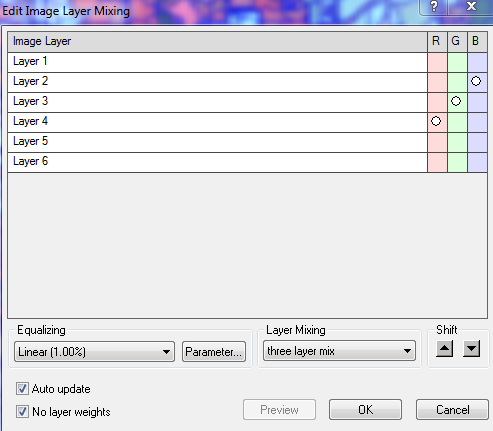
  • Method was set to IHS
  • Resampling Techniques was set to Nearest Neighbor 
  • IHS Substitution was set to Intensity
  • R = 1, G = 2, B = 3
  • Checked the box for Stretch to Unsigned 8 Bit

Apply Texture Analysis


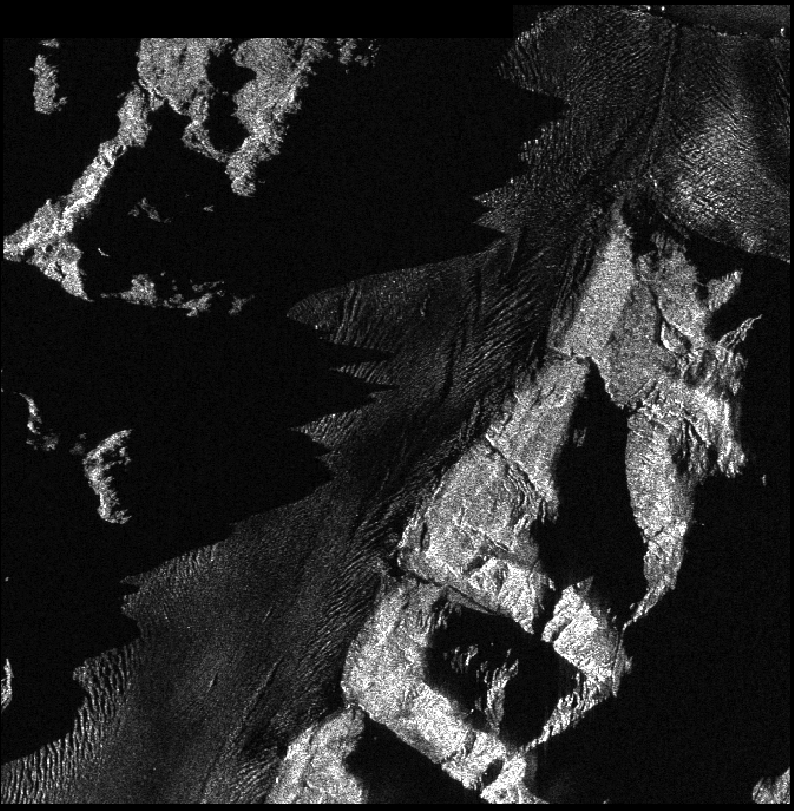
An image from Erdas Imagine example data was utilized for this section of the lab (Fig. 5)

(Fig. 5) Erdas Imagine example data radar image utilized.

I selected Texture Analysis feature from the Utilities sub-tab found under the Raster menu. In the dialog box I set the Operators to Skewness, the Window Size to 5.

Brightness Adjustment

I utilized the same image from Texture Analysis for this section of the lab.  I selected Brightness Adjustment from the Utilities sub-menu which is located under the Raster menu. The Data Type was set to Float Single and the Output Options was set to Column.    


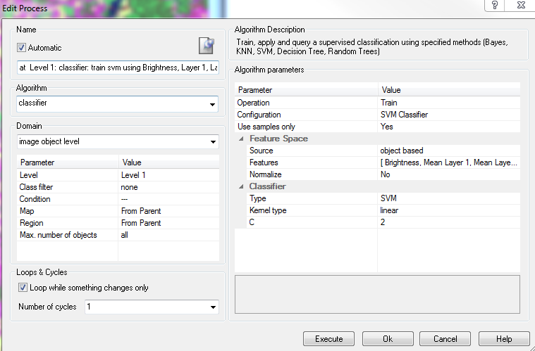
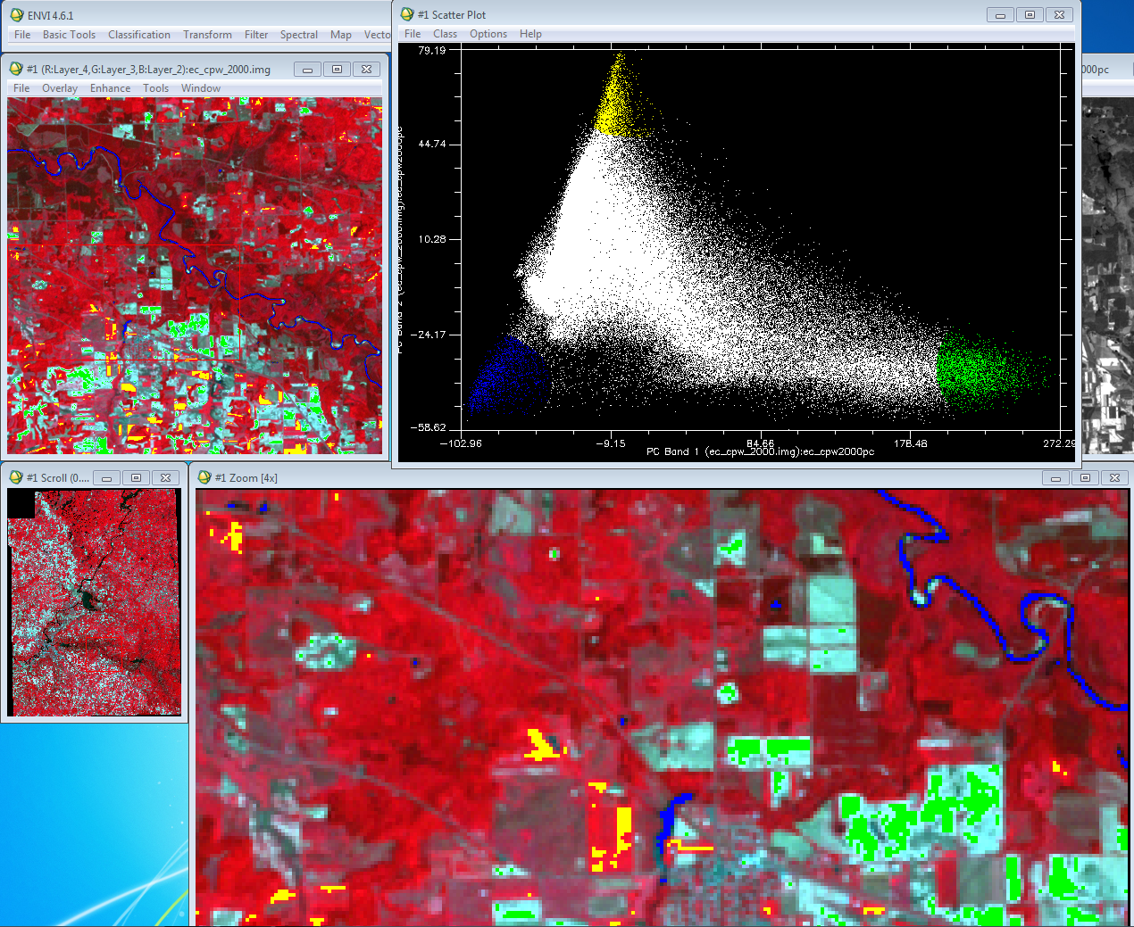
Polarimetric SAR Processing and Analysis

The remaining sections of this lab were performed in ENVI 4.6.1.

In this section of the lab I will be working with radar imagery of a section of Death Valley. The imagery was collected by the SIR-C radar system. A great amount of preprocessing was applied to the imagery before I obtained the image from my professor.
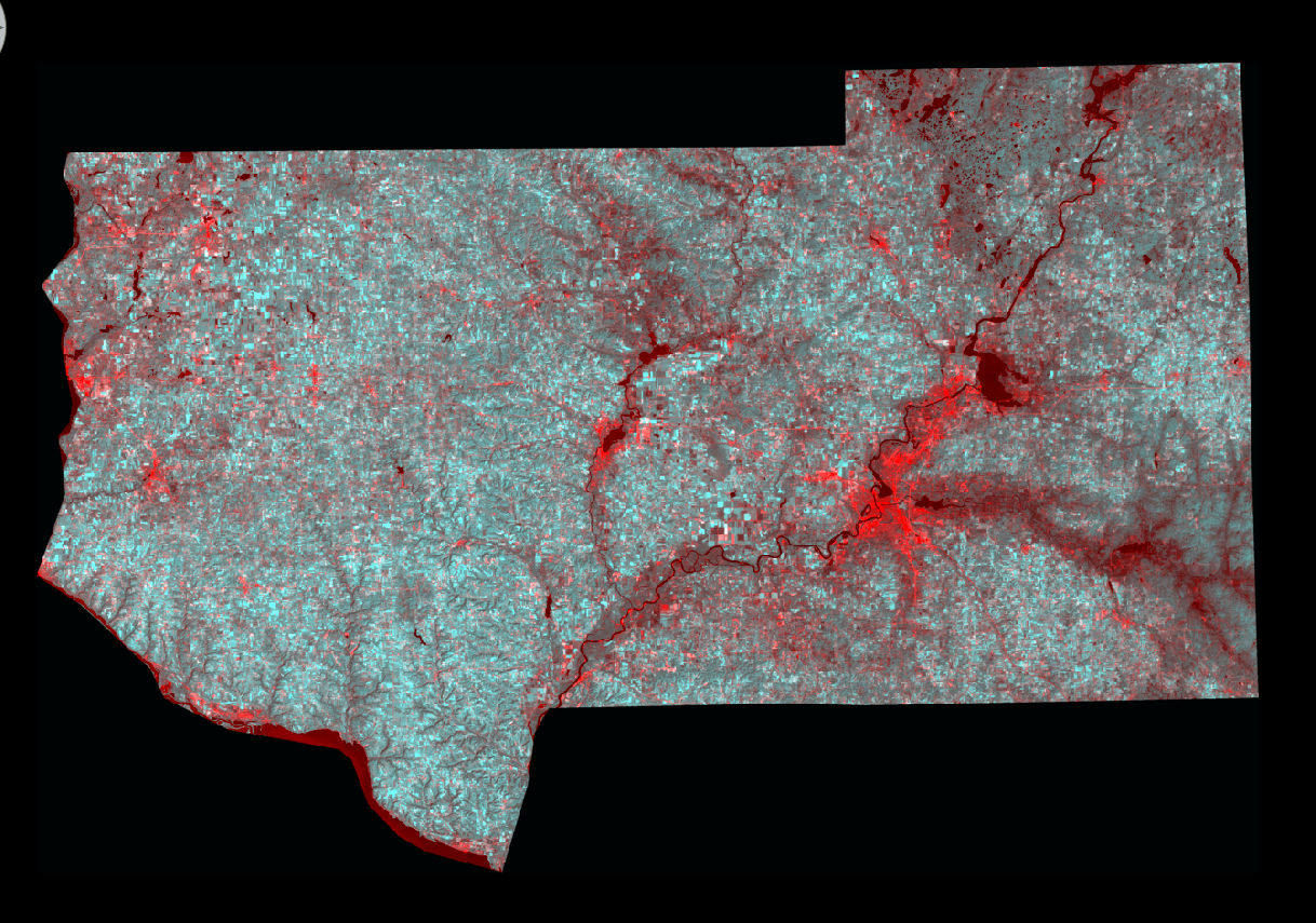
Synthesize Images

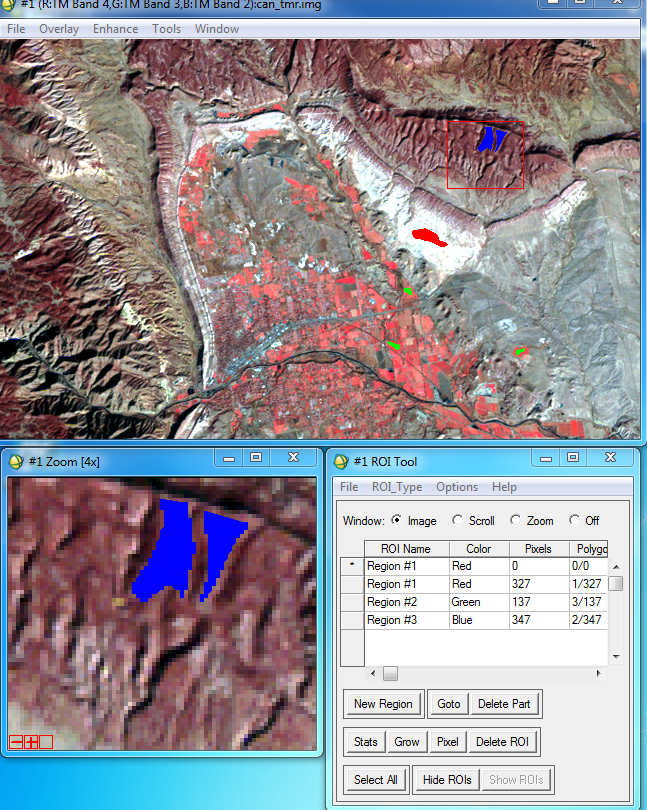
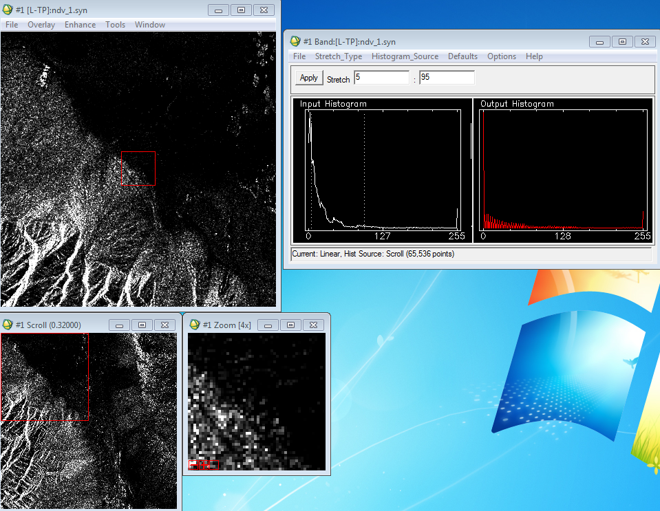
The SIR-C data I was provided was in a non-image/compressed format. To view the images I needed to mathematically synthesize the images from the compressed scattering matrix data. The first step is to select the file through the Synthesize SIR-C Data from the Polarimetric Tools sub-menu found under the main menu bar Radar menu. After opening the file the Synthesize Parameters dialog box opens (Fig. 6). Changing the Output Data Type to Byte I selected OK and the four polarization combinations were added to the Available Bands List. I then loaded one of the polarization images in to a new viewer (Fig. 7). 

(Fig. 6) Synthesize Parameters dialog box.

(Fig. 7) Death Valley image after synthesizing the images.


I then opened the images in the viewer utilizing Interactive Stretching from the Enhance menu.  I compared 3 different stretch settings including Gaussian, Linear, and Square-root. The left Stretch field was set to 5 and the right was set to 95 for all methods.

Slant-to-Ground Range Transformation

I used the same image from the previous section of Death Valley. Slant-to-Ground Range transformation is required due to the side angle at which radar data is collected. The angle does not produce a true scale representation of the ground among other distortions.  This step will correct the "ground range" of the image.

Selecting SIR-C from the Slant to Ground Range sub-menu from the Radar menu. After selecting the image and opening the file the Slant to Ground Range Parameter dialog box opens. I set the Output pixel size to 13.32, and the Resampling Method to Bilinear.

Results


(Fig. 8) Display of the speckle filter results. The original image (top left), 1st suppression (top right), 2nd suppression (bottom left), and 3rd suppression (bottom right).
(Fig. 9) Results from Edge Enhancement
(Fig. 10) Results for the Wallis_Filter (right) and original image (left).
(Fig.11) Merge results


(Fig. 12) Texture analysis results.
(Fig. 13) Brightness Enhancement results

(Fig. 14) Guassian Stretch result.
(Fig. 15) Interactive Stretch result.
(Fig. 16) Linear Stretch Result
(Fig. 17) Square Root Stretch result
(Fig. 18) Slant Range result.


Thursday, April 21, 2016

Lab 10: Advanced Classifiers 3

Goals and Background

The main purpose of the lab is to learn the processes for two new algorithms for performing advanced classification.  The lab will have me performing an expert system/decision tree classification utilizing provided ancillary data and then I will use an artificial neural network to perform complex image classification.  Throughout the following blog I will summarize the methods I used to complete the classification for both methods and display the results.

Methods

Expert System Classification

All of the methods for this section were performed in Erdas Imagine 2015.

Expert system classification is one of a limited number of classifiers which can produce results above the required accuracy requirements.  The expert system utilizes ancillary data such as zoning data or Census (population) data to assist in classifying a remotely sensed image.

I was provided an image from my professor of the Eau Claire and Chippewa Falls area in Wisconsin (Fig 1). The image has a few accuracy errors when analyzing the original classification which was performed. Certain green vegetation areas along with certain agricultural areas and a few other features have been classified incorrectly. In the following steps I will be utilizing the expert system classification method to improve the accuracy of the original classification.

(Fig. 1) Orginal classified image provided to me by my professor of the Eau Claire and Chippewa Falls area.


The first step is to develop a knowledge base by which to improve the original classified image. To accomplish this I opened the Knowledge Engineer interface from the Raster sub-menu. From the Knowledge Engineer interface I created hypothesis & rule to classify each class for the image.  The first rule I created was for water (Fig. 2).  I then created a rule for the remaining classes.

(Fig. 2) Rule Props window creating the rule for the water class.


The second step is to add the ancillary data in to the rules to assist in the classification. The first new hypothesis I created was labeled Other urban. In the Rule Props window inserted the variable provided to me by my professor which will assist the algorithm select out the "other urban" areas (Fig. 3). Then a second variable was inserted to classify the areas with the proper label in the image. The second step is to make a counter argument for the original Residential classification to exclude the residential area from being classified in to the "other urban" area (Fig. 4). I then utilized the same process to use ancillary data to convert green vegetation which was wrongly classified as agriculture and a separate hypothesis for the opposite. After completing the previous tasks the decision tree was complete and ready to perform the classification (Fig. 5).

(Fig. 3) Creation of the Other Urban area rule with tree display.

(Fig. 4) Creation of exclusion rule for the original Residential class.
(Fig. 5) Knowledge Engineer window with the decision tree completed.

Opening the Knowledge Classifier from the Knowledge Engineer menu opened the Knowledge Classification window after opening the above knowledge file in the first window (Fig. 6). Selecting next will then open up a new window to declare your output file name and parameters (Fig. 7).  The cell size was set to 30 by 30 per the instructions of my professor. The last step was to run the classification by selecting OK.

(Fig. 6) Knowledge Classification window with specified classes selected.

(Fig. 7) Knowledge Classification window with output file set.
Neural Network Classification

All of the step unless noted for this section were performed in ENVI 4.6.1.

I opened the image provided to me from my professor and displayed as 4,3,2 band combination in the viewer. I then imported an ROI file containing training samples previously collected by my professor (Fig. 8).

(Fig. 8) Original image with ROI locations overlayed in the ENVI viewer.

I then selected Neural Net from the Supervised sub-meun of Classification to open the Classification Input File window (Fig 9************).  From this window I selected the image and clicked OK to proceed to the  Neural Net Parameters window. I set the parameters according to my professors guidelines/specification (Fig. 10***********). I then ran the classification and opened the results in new viewer (Fig.11).

(Fig. 11) Results from the Neural Network classification in ENVI.
An optional portion of the lab was to create my own training samples and classifiy a QuickBird image of the University of Norther Iowa campus (Fig. 12).  I opened the provided image and created my training samples per my instructions.  I then proceeded to utilize the same procedure to complete the classification of the image (Fig. 13).


(Fig. 12) Quickbird image with display of created training samples and parameter windows.


(Fig. 13) Results of the classification for the campus image in ENVI.

Results


Sources


Thursday, April 14, 2016

Lab 9: Object Based Classification

Goals and Background
The main purpose of this lab is to gain knowledge in performing object-based classification within eCognition.  eCogniton is a computer program which only performs object-based classification of satellite images. Object-based classification is a somewhat new form of classification in the world of remote sensing.   In this lab I will learn the step required to perform object-based classification.  I will be using two different classification methods which include, random forest classifier and support vector machine classifier.

Methods
I performed both forms of classification on the same image of the Chippewa and Eau Claire County in Wisconsin from previous classification labs.  The classification process was performed in eCognition as stated above.  Additional programs will be noted for there uses.

I imported the image provided to me utilizing Import Image Layer after creating a New Project. The resolution was set to 30 /pxl and the Use geocoding box was selected. The image was displayed in an unfamiliar color scheme.  I utilized Edit Image Layer Mixing to change the color display to a familiar 4,3,2 band combination (Fig. 1).

(Fig. 1) Edit Image Layer Mixing window set to display a 4,3,2 band combination image.


Segmentation and Sample Collection

I created a new process in the Process Tree after opening from the Process menu.  The first “process” acts like a label/heading to build the “tree” from. From the first process I created a New Child which I labeled Generate objects.  The step will be creating segmentation with in the image.  Segmentation groups like features based on pixel value, texture, and compactness. In the edit window I set the Algorithm to multiresolution segmentation along with setting Shape to .3 and Compactness to .5. per the instruction of my professor.  The setting for shape and compactness were derived from trial and error from previous work my professor has done. I selected Execute after assuring all of my parameters were set correctly. The image was now displayed with the created segmented areas (Fig. 2).

(Fig. 2) Zoomed in image with the segmentation layer over top of the satellite image.


Creating training samples is the next step of the classification process. For this lab I will be creating classification for the following classes:
  • ·         Forest
  • ·         Agriculture
  • ·         Urban/Built-up
  • ·         Water
  • ·         Green vegetation/shrub
  • ·         Bare soil

Using Class Hierarchy and Insert Class I was able to create classes and label them with a corresponding color (Fig. 3). Take from Lab instructions if needed). With the classes created I was able to start collecting samples using Select Samples from the Classification menu and Samples sub-menu. I zoomed and panned around the image selecting areas which were homogeneous with forest areas after selecting Forest from the classes list. After selecting an area the segmented area would change to the color corresponding to the class (Fig.4*****************).  After collecting the required number of samples (specified by my professor) for the forest areas I utilized the same process for all the remaining classes.

(Fig. 3) Class list created for classification.

(Fig. 4) Image of sample areas selected with appropriate color displayed.


Implement object classification

I created a Scene Variable from the Manage Variable window found under the Process menu. The scene variable is like setting environments in ArcMap as it gives a location for the processing to store information.

I Appended New process labeled RF Classification below the segmentation “Level 1” step. I then inserted a New Child to the new process. The new child process was labeled Train RF Classifier.  Within the Edit Process window I set a number of parameters to properly execute the training classification (Fig. 5).  The parameters again were given to me from my instructor based on his experience with the RF Classification. The training samples were brought in to the classifier window through the Feature drop down in the Edit Process window. The Select Features window opens after selecting <select features…> from the drop down menu. I added selected parameters from my trainings samples within the window per the advice of my professor (Fig. 6*************). The final step is to implement/perform the classification. I inserted a child to RF Classification labeled Apply RF Classifier. The parameters were set in the window to properly apply the previous steps to the image (Fig. 7*****).  Select the View Classification icon after Executing the apply step of the process.

(Fig. 5) Edit Process window with parameters set to train the RF classifier.

(Fig 6) Select Features menu with training data selected.


(Fig. 7) Edit Process window applying the RF classification.


(Fig. 8) Process Tree after imputing all of the processes to perform RF Classification.


Export to Erdas

Utilizing Export Results from the Export tab I created an Erdas Imagine Image.  I opened the image in Erdas Imagine to alter the color scheme of the classification to match previously completed classifications. 

Support Vector Machines

Support Vector Machines (SVM) is another learning algorithm which utilizes a hyperplane to perform classification of segmented areas.

I utilized the same steps above to perform the SVM classification on the same segmented image. The only difference is the parameter settings when training the classifier (Fig. 9). The parameter setting were again provided to me by my professor in the lab instructions.


(Fig. 9) SVM classification parameters set in the Edit Process window.


Results


Both classification results had some error when comparing the produces map with Google Earth. The areas with errors could have been corrected using Manual Editing in eCognition.  The likely reason for the error is from incorrectly selected training samples. The SVM classification produced more accurate results compared to the RF classification from my observations.

Sources

Lta.cr.usgs.gov,. (2016). Landsat Thematic Mapper (TM) | The Long Term Archive

Thursday, April 7, 2016

Lab 8: Advanced Classifiers 1

Goals and Background

The purpose of this lab is gain knowledge and utilize spectral linear unmixing and fuzzy classification.  Spectral linear unmixing and fuzzy classification are advanced classifiers. These powerful algorithms produce more accurate results when classifying remotely sensed images compared to conventional supervised and unsupervised classification.

Methods

Spectral Linear Unmixing

For this portion of the lab I utilized Environment for Visualizing Images (ENVI) software.  I performed my spectral linear unmixing on an ETM+ image of Eau Claire and Chippewa county in the state of Wisconsin.

The Available Bands List opens after opening your image file in the ENVI 4.6.1 software. From the window I set the RGB Color scheme to a 4,3,2 band combination (Fig. 1). The image will be displayed in 3 different windows of varying zoom levels after selecting Load RGB button from the list.

(Fig. 1) Available bands list in ENVI

First, I had to convert the image to principle component before running the spectral linear unmixing. Principle component removes the noise from the original image which helps improve the accuracy during the unmixing process. Accessing Compute New Statistics and Rotate from the Transform menu I was able to convert the original image to Principal Component. After opening the PC image created in the previous step the Available Bands List now contains six PC band images.

I moved the zoom window around till I found an area with agriculture, bare soil, and water contained in the viewer. Next I opened the scatter plots for PC Band 1 and PC Band 2. Select 2-D Scatter Plots from the Tools menu to open the The Scatter Plot Band Choice window.  I then selected PC Band 1 for X and PC Band 2 for Y.

With the scatter plot display I collected my end-member sample.  The end-member sample contains "true" samples for a given class. When drawing the polygon/circle for the end-member selection you don't know what class (land cover type) you are selecting. I selected Item 1:20 from the Class menu and then I selected Green Color.  I then drew a circle around one of the ends of the triangle and right mouse clicked inside the circle to finish my selection (Fig. 2).  Once I finished the selection the sample areas turned green on the image depicting the area I had selected.  In (Fig. 2) I had selected the bare soil end member.  I completed the same process but changed the color for each of the other end members (Fig. 3).  The other 2 end members contained agriculture areas and water.

(Fig. 2) Collecting of the first end member from the scatter plot.
(Fig. 3) Completed collecting the other end member samples from the scatter plot.
The next objective of the lab was to located the urban area from the scatter plots.  I loaded PC 3 and PC 4 with the same process as before.  The scatter plot was not as triangular like other plots.  I search around till I found the area of the scatter plot which contained the urban/built up areas (Fig. 4). 

(Fig. 4) Selection from the scatter plot displaying urban/built up area.
After collecting the end member I saved the ROIs in preparation for implementing Linear Spectral Mixing. I then opening Linear Spectral Mixing from the Spectral tab. Utilizing the orginal image and the ROIs from the previous step I created fraction images displaying the various land covers (Fig 5).

(Fig. 5) Fractional images created from the Linear Spectral Mixing. The brighter (white) the area the more suitable the reflectance for the specific class.  (Left to right) Bare soil, Water, Forest, Urban/Built up.

The fractional images can be utilized to create a classification image.  For the purposes of this lab I will not be creating a classification image from the fractional images.  In order to create a classified image I would need to collect the 5th end member to give me the 5 LULC classes I have been creating in previous labs.

Fuzzy Classification

The process of fuzzy classification was performed in Erdas Imagine.

Fuzzy classification is like a advanced version of supervised classification. The classification method has the ability to break the pixel down to different classes (Fig. 6). Breaking down the pixel allows for more accurate classification of remotely sensed images.

( Fig. 6) The ability for Fuzzy classification to break a single pixel to individual classes.
I collected training samples the same way I did in Lab 5. One difference when collecting training samples for fuzzy classification you want to collect an equal number of homogeneous samples and heterogeneous samples. The collection of both types of samples is a better representation of the real world and results in more accurate classification.  After collecting the signature I merged the files as I did in lab 5.

To perform fuzzy classification I opened the Supervised Classification window.  I input the proper files including my signature file and distance file I created in the previous step. I utilized Maximum Likelihood as the Parametric Rule.  I changed the Best Classes Per Pixel to 5 and then proceeded to run fuzzy classification.   I selected  Fuzzy Convolve to combine the results to make one image.  I tooked the combined image and created a map in ArcMap (Fig 7).


(Fig. 7) Classified image using fuzzy classification.


Sources

Lta.cr.usgs.gov,. (2016). Landsat Thematic Mapper (TM) | The Long Term Archive


Friday, March 25, 2016

Lab 7: Digital Change Detection

Goals and Background

The purpose of this lab is to gain knowledge and skills in measuring and identifying change of LULC over a specified time period utilizing remotely sensed imagery.  I will be conducting a quick qualitative change detection method along with a quantifying post-classification changed detection method.  Additionally, I will be creating a model which will allow me to display the result of the change detection on a map.

Methods

All of the following step were performed in Erdas Imagine 2015.

Change detection using Write Function Memory Insertion

Utilizing Write Function Memory Insertion is a simple yet powerful method to detect changes between images of the same area from different time frames. The analyst simply opens the near-infrared bands from the two dates of imagery in the red, green, and blue color guns.  The pixles within the images which have changed will be displayed as a different color against those which remained the same.

For this section of the lab I utilized images of Eau Claire and surrounding counties provided to me by my professor Dr. Wilson.  I opened the an image containing the red band (band 3) from 2011 and then 2 images of near-infrared band of the same area from 1991.  The last step was to layer stack the images together.  I opened the layer stacked image in a viewer in Erdas to see the results (Fig. 1).

(Fig. 1) Results from performing Write Function Memory Insertion.  The bright red areas are where change has occurred in the images between the two dates.

Post-classification comparison change detection

For this section of the lab I will be conduction change detection of the Milwaukee Metropolitan Statistical Area (MSA) between 2001 and 2011.  I was provided previously classified images from my professor Dr. Wilson.

The first objective for this section of the lab is to quantify the change which has occurred in the Milwaukee MSA in hectares between the classified image from 2001 and classified image from 2011. I brought the two image in to separate viewers in Erdas (Fig. 2).

(Fig. 2) 2001 classified image (Left) and 2011 classified image (Right) of the Milwaukee MSA in Erdas.
The next step was to obtain the histogram values from the raster attribute table and input the values in to an Excel spreadsheet with the proper classes (Fig 1).  The next step was to convert the histogram values to square meters and then to hectares.

(Fig. 3) Histogram values input in to Excel spreadsheet converted to Hectares.
Once the values were converted into Hectares I was able to calculate the percent of change for each class for the Milwaukee MSA area (Fig. 4).

(Fig. 4) Percent change between the 2001 and 2011 image of the Milwaukee MSA area.


The next step for this section of the lab is to develop a From-to change map from the two images.  I created a model to detect the change between the two images.  Within the model I will also create an image which displays the areas which have changed for the following classes.

  1. Agriculture to urban/built-up
  2. Wetlands to urban/built-up
  3. Forest to urban/built-up
  4. Wetlands to agriculture
  5. Agriculture to bare soil

I will be utilizing the Wilson-Lula algorithm to detect the change and create the display images.  The first step is to separate the individual classes using an "either or" statement.  The either or statement will create a image containing one class only, such as, agriculture areas and nothing else. Each separate class is grouped together to match the above list of five comparative classes.  The "either or" images was put into a temporary raster to save on storage space within the computer.  The next step was to use a Bitwise function to shows the areas which changed from one LULC class to another. The output from the function can be input on a map to display the areas of change.

(Fig 5) Model utilizing the Wilson-Lula algorithm.

Results


(Fig. 6) Map displaying the LULC change in the Milwaukee MSA area.
Sources

Homer, C., Dewitz, J., Fry, J., Coan, M., Hossain, N., Larson, C., Herold, N., McKerrow, A., VanDriel, J.N., and Wickham, J. 2007. Completion of the 2001 National Land Cover Database for the Conterminous United States.Photogrammetric Engineering and Remote Sensing, Vol. 73, No. 4, pp 337-341.

Xian, G., Homer, C., Dewitz, J., Fry, J., Hossain, N., and Wickham, J., 2011. The change of impervious surface area between 2001 and 2006 in the conterminous United States. Photogrammetric Engineering and Remote Sensing, Vol. 77(8): 758-762.