Lab 8: Advanced Classifiers 1

Goals and Background

The purpose of this lab is gain knowledge and utilize spectral linear unmixing and fuzzy classification.  Spectral linear unmixing and fuzzy classification are advanced classifiers. These powerful algorithms produce more accurate results when classifying remotely sensed images compared to conventional supervised and unsupervised classification.

Methods

Spectral Linear Unmixing

For this portion of the lab I utilized Environment for Visualizing Images (ENVI) software.  I performed my spectral linear unmixing on an ETM+ image of Eau Claire and Chippewa county in the state of Wisconsin.

The Available Bands List opens after opening your image file in the ENVI 4.6.1 software. From the window I set the RGB Color scheme to a 4,3,2 band combination (Fig. 1). The image will be displayed in 3 different windows of varying zoom levels after selecting Load RGB button from the list.

(Fig. 1) Available bands list in ENVI

First, I had to convert the image to principle component before running the spectral linear unmixing. Principle component removes the noise from the original image which helps improve the accuracy during the unmixing process. Accessing Compute New Statistics and Rotate from the Transform menu I was able to convert the original image to Principal Component. After opening the PC image created in the previous step the Available Bands List now contains six PC band images.

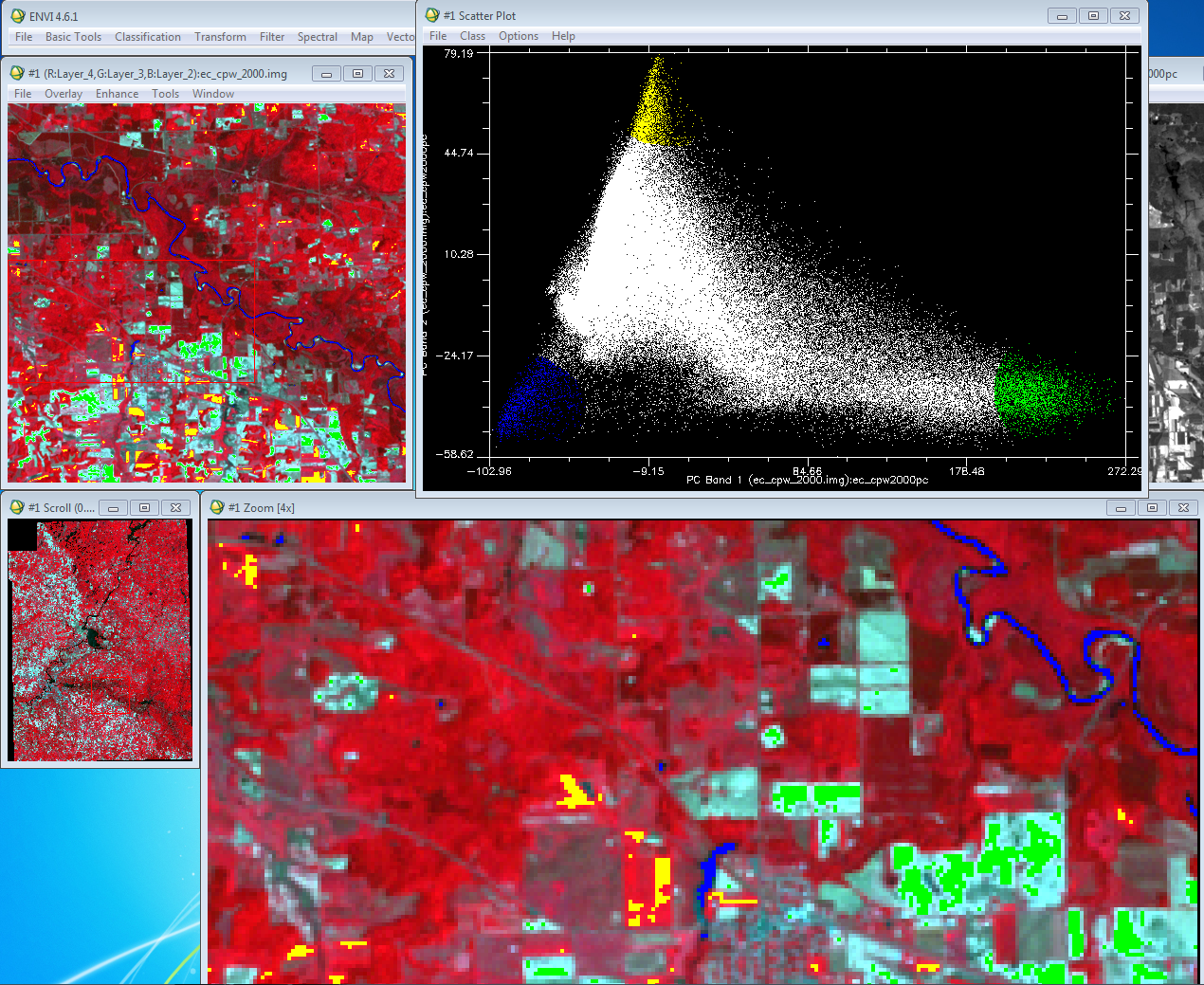
I moved the zoom window around till I found an area with agriculture, bare soil, and water contained in the viewer. Next I opened the scatter plots for PC Band 1 and PC Band 2. Select 2-D Scatter Plots from the Tools menu to open the The Scatter Plot Band Choice window.  I then selected PC Band 1 for X and PC Band 2 for Y.

With the scatter plot display I collected my end-member sample.  The end-member sample contains "true" samples for a given class. When drawing the polygon/circle for the end-member selection you don't know what class (land cover type) you are selecting. I selected Item 1:20 from the Class menu and then I selected Green Color.  I then drew a circle around one of the ends of the triangle and right mouse clicked inside the circle to finish my selection (Fig. 2).  Once I finished the selection the sample areas turned green on the image depicting the area I had selected.  In (Fig. 2) I had selected the bare soil end member.  I completed the same process but changed the color for each of the other end members (Fig. 3).  The other 2 end members contained agriculture areas and water.

(Fig. 2) Collecting of the first end member from the scatter plot.

(Fig. 3) Completed collecting the other end member samples from the scatter plot.

The next objective of the lab was to located the urban area from the scatter plots.  I loaded PC 3 and PC 4 with the same process as before.  The scatter plot was not as triangular like other plots.  I search around till I found the area of the scatter plot which contained the urban/built up areas (Fig. 4). 

(Fig. 4) Selection from the scatter plot displaying urban/built up area.

After collecting the end member I saved the ROIs in preparation for implementing Linear Spectral Mixing. I then opening Linear Spectral Mixing from the Spectral tab. Utilizing the orginal image and the ROIs from the previous step I created fraction images displaying the various land covers (Fig 5).

(Fig. 5) Fractional images created from the Linear Spectral Mixing. The brighter (white) the area the more suitable the reflectance for the specific class.  (Left to right) Bare soil, Water, Forest, Urban/Built up.

The fractional images can be utilized to create a classification image.  For the purposes of this lab I will not be creating a classification image from the fractional images.  In order to create a classified image I would need to collect the 5th end member to give me the 5 LULC classes I have been creating in previous labs.

Fuzzy Classification

The process of fuzzy classification was performed in Erdas Imagine.

Fuzzy classification is like a advanced version of supervised classification. The classification method has the ability to break the pixel down to different classes (Fig. 6). Breaking down the pixel allows for more accurate classification of remotely sensed images.

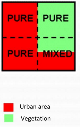( Fig. 6) The ability for Fuzzy classification to break a single pixel to individual classes.

I collected training samples the same way I did in Lab 5. One difference when collecting training samples for fuzzy classification you want to collect an equal number of homogeneous samples and heterogeneous samples. The collection of both types of samples is a better representation of the real world and results in more accurate classification.  After collecting the signature I merged the files as I did in lab 5.

To perform fuzzy classification I opened the Supervised Classification window.  I input the proper files including my signature file and distance file I created in the previous step. I utilized Maximum Likelihood as the Parametric Rule.  I changed the Best Classes Per Pixel to 5 and then proceeded to run fuzzy classification.   I selected  Fuzzy Convolve to combine the results to make one image.  I tooked the combined image and created a map in ArcMap (Fig 7).

(Fig. 7) Classified image using fuzzy classification.

Sources

Lta.cr.usgs.gov,. (2016). Landsat Thematic Mapper (TM) | The Long Term Archive.