Lab 5: Pixel-based Supervised Classification

Goals and Background

The main purpose of this lab is to gain an understanding of pixel-based supervised classification to produce and land use/land cover (LULC) display.  I as the analyst will be extracting biophysical and sociocultural information from remotely sensed images to perform the classification.  I will be developing my skills in selecting and evaluating training samples to be used in supervised classification. Producing an useful display of the land use/land cover classes will be my final step in the lab.

Methods

All of the following sets were performed in Erdas Imagine unless otherwise stated.

I will be performing supervised classification on the same image of Chippewa and Eau Claire county from my previous blog post to which I performed unsupervised classification to.

Utilizing supervised classification requires more user input in the beginning from the analyst compared to unsupervised classification.  However, when creating the classes supervised classification requires little to no input from the analyst.

Designing a categorized outline for your fields is the first step in creating a classification. For this image I will be classifying the image into the following 5 categories:

1. Water
2. Forest
3. Agriculture
4. Urban/Built Up
5. Bare Soil

Collecting training samples is the next step in supervised classification.  I will be gathering spectral signatures to create the training samples to classify the image. I will be collecting multiple training samples from each class as no feature in a LULC has the same spectral signature. I will be using the Signature Editor (Fig. 1). (For more information about collecting samples the Signature Editor see my previous blog post on collecting spectral signatures.)  Making sure you are collecting a sample from one form of LULC is essential to collecting an accurate training sample.  For example you can not collect one sample from an area which contains a soy bean field and a corn field.  Though both types of the fields would fall under the agricultural LULC having a mixed training sample with affect your final results. I utilized the Google Earth Sync feature as I have in the past few blogs to assist me in identifying LULC class areas.

(Fig. 1) Collecting training samples using the Signature Editor.

I collected between 12-20 samples per LULC class.  When I felt I had a good distribution across the image and had collected samples from the majority of the different surfaces I ceased taking samples for the particular class.  I collected a total of 83 signatures across all of the LULC classes when I finished collecting samples.

Evaluating the quality of training samples.

The next step is to evaluate the quality of the training samples I collected.  Examining all the spectral signatures of one class in the Signature Mean Plot window viewer gave me an overview of all the signatures in a class (Fig. 2).  Examining the displayed plots shows a pattern or trend between the spectral signatures.  Additionally, the displayed plots display signatures which do not follow the same pattern.  Within Fig. 2 I have displayed the signatures which do not follow the pattern in gold.

(Fig. 2) Display of spectral signatures for the urban samples I collected.  Signatures following the correct patter are in aqua and the questionable signatures are displayed in gold.

I needed to examine the histogram display for all the bands of the signature for the each questionable samples individually.  The examination of the histogram will help me to determine if the sample can be utilized as a training sample.  When analyzing the histograms I was looking to see if more than 4 of the histograms from each sample were multimodal (Fig. 3). If more than 4 of the histograms were mulitmodal then the sample must be deleted and not utilized in the supervised classification. Four or more multimodal histograms tell the analyst he/she collected a sample from more than one type of land cover such as a soy bean field and a spruce forest.

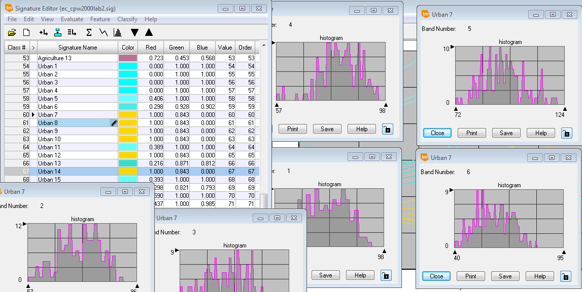(Fig,. 3) Display of a sample with all the histograms from all the bands being multimodal.

Having the one histogram from all the bands displayed as multimodal is acceptable and the signature can still be utilized for supervised classification (Fig. 4).

(Fig. 4) Display of a sample with all but one histogram from all the band being non-multimodal.

After eliminating the signatures which were not accurately collected I displayed all of he signature on one Spectral Mean Plot window (Fig. 5).  I was left with 77 signatures when I completed deleting the erroneous results.

(Fig. 5)  Spectral Mean Plot window with all of the remaining signature plots.

The next step in the accuracy assessment is to assure the five informational class signatures do not overlap in more than four bands.  I performed a separability analysis to assess which bands will give me the best spectral separability.  Selecting Separability from the Evaluate tab opened the Signature Separability window (Fig. 6).  I changed the Layers Per Combination to 4 and the Distance Measure to Transformed Divergence and left the other settings alone and ran the evaluation.

(Fig. 6) Signature Separability settings window in Erdas Imagine. 

A report is generated when the evaluation is complete (Fig. 7).  Scrolling down a number of pages will bring you to the a list of the four bands which have the best average separability based on the collected signatures.  Then the Best Average Separability value is listed after the four bands. The Best Average Separability value should be above 1900 to have good separability.  Excellent separability is a score above 2000.  Any score below 1700 is in accurate and training samples need to be collected again in a more accurate manner.  Bands 1,2,4,5 are the bands with the best separability and my Best Average Separability value is 1960 for my signatures I collected.

(Fig. 7) Separability report, with bands 1,2,4,5 having the best separability and  Best Average Separability value of 1960.

Merging the individual signatures for each informational class to form one signature for that class is the final step before running the supervised classification.  Highlighting all of the signatures for one class and selecting Merge from the Edit menu will produce a single signature to represent the class. I repeated this step for all of the classes.  I deleted all of the individual signatures which left me with 5 spectral signatures in the Signature Editor window (Fig. 8). I saved this signature file for use in the classification.

(Fig. 8) Signature Editor window with 5 classes after merging the individual signatures into one signature.

Plotting these results in the Signature Mean Plot window makes it easier to see the separability between the bands (Fig. 9).

(Fig. 9) Signature Mean Plot of the merged spectral samples.

Performing supervised classification

Performing the supervised classification is very simple once all of the preparation work is completed. Selecting Supervised Classification from the Supervised sub-tab from the Raster menu will open up the classification settings window (Fig. 10).  The Input Raster File is the base satellite image, and the Input Signature File is the signature file I save from the Merge operation above.  The Classified File  is your output image/classification.  I did not change the default settings under Decision Rules and proceeded to run the supervised classification.  

(Fig. 10) Supervised Classification settings window.

Results

(Fig. 11) Display of my supervised classification results.

The results from the supervised classification are more accurate than the unsupervised classification from the last weeks lab for all the areas except the Urban areas.  Many agricultural fields and bare soil areas were given labels of Urban areas.  The extensive variation between urban surfaces makes it the most difficult class to properly classify.  I am certain more diverse training samples from urban areas would lead to more accurate results.

Sources

Lta.cr.usgs.gov,. (2016). Landsat Thematic Mapper (TM) | The Long Term Archive.