The main purpose of this lab is to learn the proper skills of extracting land surface temperatures from thermal bands of various satellite images. In this lab I will be visually identifying variations in land surface temperature and utilizing models to convert the Digital Number (DN) to at-satellite radiance and at-satellite radiance to blackbody surface temperature across various collected satellite images.
Methods
All of the following methods unless noted were performed in Erdas Imagine 2015.
Visual Identification of Relative Variations in Land Surface Temperature
The first task of the lab was to compare tonal differences between band 61 (high grain) and band 62 (low grain). You can see in (Fig.1) there are only slight variations between the two bands. Band 61 has lighter tones or appears to be more washed out and contrast less between the dark and light tones. Band 62 has greater variation in the tones and it more easily understood by the reader. The darker the tone the cooler the surface temperature.
 |
| (Fig. 1) High Grain Band 61 (Left) & Low Grain Band 62 (Right) ETM+ images |
When obtaining thermal satellite images the values are stored as a Digital Number (DN). Converting the DN to kinetic (true) surface temperature requires a three stage process. The first step is to convert the DN to "at-satellite radiance". This step removes outgoing atmospheric interference from the image. The formula to achieve to conversion is Grescale * DN + Brescale.
Conversion of Digital Numbers (DN) to at-satellite radiance
The first step in the process is to calculate the Grescale. To calculate Grescale you need to obtain LMAX, LMIN, and QCALMAX, and QCALMIN from the metadata of the image. The formula to calculate Grescale is (LMAX-LMIN)/(QCALMAX-QCALMIN).
The second step to identify Brescale which is equal to LMIN.
The final step is to input the previous information into the formula (Grescale * DN + Brescale).
To practice this process I utilized the band 62 image from the Visual Identification section.
I consulted the metadata and proceeded to calculate Grescale and identify Brescale which allowed be to create a model utilizing the final formula to convert the image from DN to at-satellite radiance (Fig. 2)
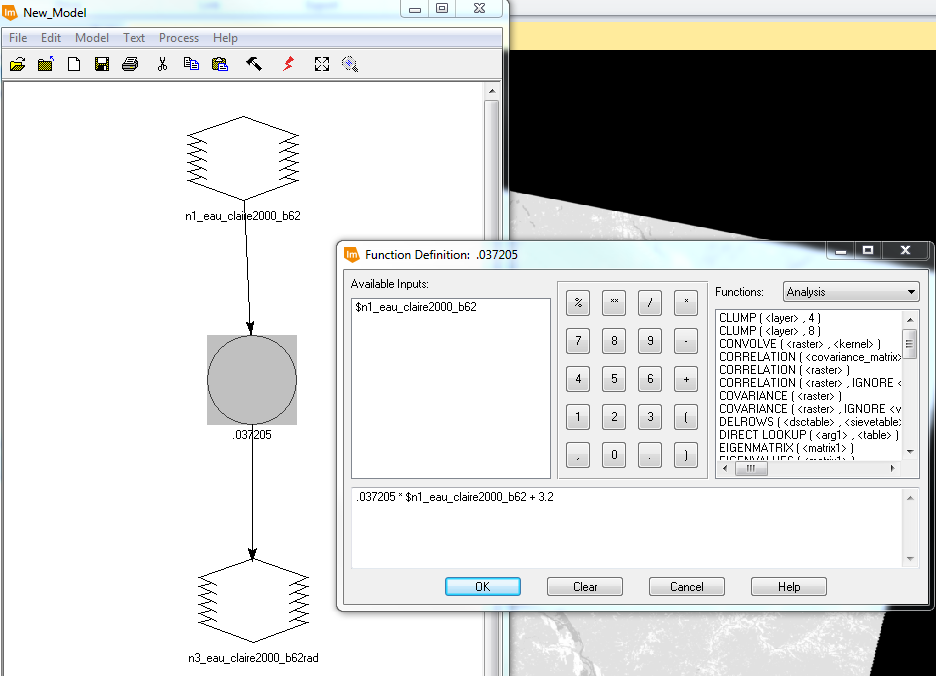 |
| (Fig. 2) Formula input into model to convert original image to at-satellite radiance. |
Conversion of At-Satellite Radiance to Blackbody Surface Temperature
The next step to obtain kinetic temperatures is to apply another formula to the image create in the previous step. The formula results in at-satellite temperatures in kelvin = K2/LOG (K1/Previous Image +1). I was provided K1 and K2 in a chart by my professor (Fig. 3). I created a model utilizing the formula to convert the previous image from at-satellite radiance to Blackbody surface temperature (Fig. 4).
 |
| (Fig. 3) K1 and K2 chart. |
 |
| (Fig. 4) Formula input into model to converting at-satellite image to blackbody surface temperature. |
Conversion of Radiant Temperature to Kinetic Temperature.
The last step to converting the original satellite image to kinetic temperature is to calculate emissivity and enter it into another formula (Fig.5). I will not be performing this calculation during this lab assignment.
 |
| (Fig. 5) Radiant temperature to kinetic surface temperature conversion formula. |
Complex Models
The next step in my lab was to take the simple models I had created in the previous steps and combine them into one complex model. The complex model will allow me to preform both calculations in one model which will result in one final output. I was given 2 images to hone my skills on. I will be displaying my methods for the Landsat 8 image (Fig 6). I need to perform the same processes to the image as before. However, the data is displayed a bit different in the metadata and I will be utilizing band 10 from Landsat 8 instead of 6 like the ETM+ image.
 |
| (Fig. 6) Original band 10 image from Landsat 8. |
The first step was to create a subset section of the image. I was give an AOI to create the subset from. To see the steps require to create a subset see my previous blog post.
Next I consulted the metadata and obtained all of the information needed to calculate Grescale. Instead of obtaining LMIN, I had to look for RADIANCE_MINIMUM_BAND_10. Additionally, I had to look for QUANTIZED_CAL_MIN_BAND_10 instead of QCALMIN. The previous terms are interchangeable. The same went for the "max" values for both L and QCAL.
With all the necessary information I created my model to calculate at-satellite radiance and convert the result to blackbody surface temperature. (Fig. 7). One of the advantages of creating a complex model is in calculating the Grescale you can set the output to a temporary raster file and then apply the second formula and obtain my output. This will help reduce unneeded files on the computer. From the temporary file I applied the formula to calculate blackbody surface temperature. With a simple click of the run button in the model builder I had completed both calculation with one streamlined process.
 |
| (Fig. 7) Complex model created for Landsat 8 image. |
 |
| (Fig. 8) Formula calculation at-satellite radiance. |
 |
| (Fig. 9) Formula calculation to convert at-satellite radiance to blackbody surface temperature. |
After running the model I opened the .tif file in ArcMap and created a map to display my results (Fig. 10). I changed the symbology and classification scheme to allow for better interpretation of the image.
Results
 |
| (Fig. 10) Map display of subset image and blackbody surface temperatures. |
No comments:
Post a Comment